E(X) = ![]() x ƒ(x) (discrete case)
x ƒ(x) (discrete case)
E(X) = ![]() x ƒ(x)dx (continuous case)
x ƒ(x)dx (continuous case)
Xn = 1/n ![]() Xi → as n → ∞ → E(X) ∈ ℝ
Xi → as n → ∞ → E(X) ∈ ℝ
iid~X
Tuesday, 2013 08 13 Includes some Q & A
E (expectation) is Linear
E(XY) = E(X)E(Y) (If E(XY) ∥ E(X)E(Y))
E(X) = 1/p (proof last class)
(Bernoulli trials until rth success.)
X![]() Yk (Yk are iid~Geom(p))
Yk (Yk are iid~Geom(p))
(A Representation is way to write an iid as a sum of iid)
E(X) = E(![]() Yk =
Yk = ![]() E(Yk) = r • E(Y1) = r • 1/p = r/p
E(Yk) = r • E(Y1) = r • 1/p = r/p
(Counts the # of successes in n B-trials)
Indicators...
Ik = { 1, if kth trial is a win }
Ik = { 0, if kth trial is a loss }
X = ![]() Ik (Ik is iid~ ←(0)--(1)→)
Ik (Ik is iid~ ←(0)--(1)→)
instead of 0 and 1 , it's 1-P and P νI1
E(X) = E(![]() Ik) =
Ik) = ![]() E(Ik) = n • E(I1) = n • { 1 • p + 0 • ( 1 - p ) } = n • p
E(Ik) = n • E(I1) = n • { 1 • p + 0 • ( 1 - p ) } = n • p
E(X) = ![]() x • ƒ(x) =
x • ƒ(x) = ![]() k • e-λ • (λk)/(k!) = e-λ
k • e-λ • (λk)/(k!) = e-λ ![]() (λk)/(k-1)!
(λk)/(k-1)!
λ e-λ ![]() (λk-1)/(k-1)!
(λk-1)/(k-1)!
Let j = k-1
λ e-λ ![]() (λj)/j!
(λj)/j!
= λ e-λ • eλ = λ
In E(X) ∈ ℝ, this is sometimes called the "mean" of X
You could call it the population mean
This will be represented by μ
Old def: X has Poisson Distribution with parameter λ > 0
is now...
def: X has Poisson Distribution with mean λ > 0
GEOMETRIC SERIES and EXPONENTIAL SERIES!
E(X) = (a+b)/2 ← already done
E(X) = 1/λ... Recall that half-life is ln(2)/λ
 |
| Figure 1: (See Saws) Notice that See-saw B has more of a "Spread" than See-saw A |
X - E(X) : is the deviation of X from its' mean
X-E(X) = E[X] - E[E(X)] = E(X)-E(X) = 0
To prevent this cancellation of positive deviations by negative deviations, let's square the deviations.
Definition: The Variance of X (var(X)) is the expectation of the square of the difference between the E[{X-E(X)}2] and its mean, written σ2
Definition: Standard deviation = √(σ2) = stdev(X) = √(var(X))
σ has the same units as X so σ is better for applications, whereas var(X) is better for theory (because var(X) has better properties)
var(X) = E[{X-E(X)}2] = E[{X-μ}2] = E[(X-μ)2] = E[X2-2μX + μ2] = E(X2) - 2μE(X) + μ2 = E(X2) - 2μμ + μ2 = E(X2) - 2 μ2 + μ2 = E(X2) - μ2 = E(X2) - (E(X))2
var(X+C) = var(X)
var(X+C)= E[[X+C-μX+C]2] = E[[X+C-(μX+C)]2] = E[(X-μ)2] = var(X) See #1
σX+C = σX
var(cX) = E({cX - μcX }2] = E[{cX - cμX}2] = E[c2 {X-μX}2] = c2 var(X)
⇒ stdev(cX) = √(var(cX)) = √(c2 var(X)) = |c| • stdev(X)
stdev(X) = ?
stdev(X) = √(var(X))
Use the computing Formula
var(X) = E(X2) - (E(X)2)
√(E(X2) - (E(X)2)) = √((91/6) - (7/2)2) = √((182-147)/12) = √(35/12) = $1.71
get stdev(X)
for the second one the answer will be σx = 1/λ
(X,Y) rv μx = E(X), μy = E(Y), σx2 = var(X), σy2 = var(Y)
σX+Y2 = Variance of (X+Y)
in theory... σX+Y2 = E[{(X+Y) - μX+Y}2]
=E[{X-μX + Y - μY }2 ]
=E[((X-μX) + (Y-μY))2 ]
=E[(x-μX)2 + (Y-μY)2 + 2(X-μX)(Y-μY)]
=E((x-μX)2 ) + E((Y-μY)2) + 2 • E((X-μX)(Y-μY))
=var(X) + var(Y) + 2•E((X-μX)(Y-μY))
E((X-μX)(Y-μY)) = cov(X,Y)
page 2 & 3Definition: (X,Y) r.v. the covariance of (X,Y) is cov(X,Y) = E[(X-μX)(Y-μY)]
cov(X,Y) is written as σX,Y
Note: cov(X,X) = var(X) = σX2
Note: var(X+Y) = var(X) + var(Y) + 2•cov(X,Y)
σ2X+Y = σ2X + σ2Y + 2 • σX,Y
Note: a this is a computational formula for X,Y
cov measures the way X & Y cooperate
E[(X-μX)(Y - μY) = E( XY - μY X - μX Y + μX μY ) = E(XY) - μY E(X) - μX E(Y) + μX μY
Remember... E(X) = μX and E(Y) = μY
E(XY) - μX μY = E(XY) - E(X)E(Y)
σX,Y = μXY - μX μY
Note: If X∥Y then cov(X,Y) = E(XY) - E(X)E(Y) ⇒ using ∥, E(X)E(Y) - E(X)E(Y)=0, so ∥
Hence if X∥Y ⇒ var(X+Y) = var(X) + var(Y)
var(X) = var(![]() Ik) (∥) =
Ik) (∥) = ![]() var(Ik) = n • var(I1) = ...
var(Ik) = n • var(I1) = ...
... = n[ E(I12) - (E(I1))2 ] = ...
... = n[ E(I1) - (E(I1)2] = ...
... = n[p - p2] = np( 1 - p )
var(X) = an ad hoc (latin: "for this") formula for variance
var(X) = E[X(X-1)] + E(X) - (E(X))2
E(X) = 1/p
![]() x(x-1), ƒ(x) =
x(x-1), ƒ(x) = ![]() k(k-1)p(1-p)k-1 = p
k(k-1)p(1-p)k-1 = p![]() k(k-1)qk-1 = ...
k(k-1)qk-1 = ...
... = pq![]() k(k-1)qk-2 = pq
k(k-1)qk-2 = pq![]() d2/(dq2) (qk) = ...
d2/(dq2) (qk) = ...
... = pq d2/(dq2) ![]() qk = pq d2/(dq2) (1/(1-q)) = ...
qk = pq d2/(dq2) (1/(1-q)) = ...
... = pq d2/(dq2) (1-q)-1) = pq • 2(1-q)-3
= (2(1-p))/(p2)Thus var(X) = (2(1-p))/(p2) + 1/p - (1/p)2 = ...
... = (2-2p+p-1)/(p2) = (1-p)/(p2) = failure/success2
var(X) = var(![]() Yk) =
Yk) = ![]() var(Yk) = r • var(Y1) = r • (1-p)/(p2)
var(Yk) = r • var(Y1) = r • (1-p)/(p2)
σX = √(r) • σY1
HW: Fair N-Sided Die Roll, find σX
rv X has Standardized Form XST = (X-μX)/σx
This is the z-score
NOTES:
XST > 0 ⇔ X above average
XST = 0 ⇔ X is average
XST < 0 ⇔ X below average
XST has no units (thus, it's independent of units of X)
Let X, X1, X2, X3, ... , Xn be iid
Let μ = μx
Let σ = σx
Let Xn = 1/n • ![]() Xi = sample mean Xn → E(X) = μ as n → ∞
Xi = sample mean Xn → E(X) = μ as n → ∞
XnST = E(Xn) = E( 1/n • ![]() Xi] = 1/n •
Xi] = 1/n • ![]() E(Xi)
E(Xi)
By iid E(Xi)'s are all the same, so...
= 1/n • n • μ = μ = μX
so:
XnST = μX
Z-Score: XnST = (Xn - μX)/( σX / √(n) )
Let X, X1, X2, X3, ... iid, μ = E(X), σ2 = var(X) Xn = 1/n • ![]() Xi
Xi
-∞ ≤ a ≤ b ≤ ∞ ⇒ ![]() P( a < (Xn-μ)/(σ/√(n)) < b ) = ...
P( a < (Xn-μ)/(σ/√(n)) < b ) = ...

 dx = XnST
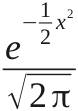
Thus, for a large n, XnST acts (roughly) as if it had pdf φ(x) = , x ∈ ℝ
(The proof of this is in MAT807, next Summer)
Note, y = φ(x) has as its graph, the famous "Bell Curve"
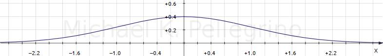 |
| Figure 2: The Bell Curve |
HW: find y' and y''
Recall, pdf density is ƒ and cdf is F
The cdf Φ(t) = 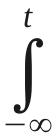 φ(x) dx = dx = ...
| When t ≥ 0 | When t < 0 |
|---|---|
1/2 +  dx dx | 1/2 -  dx dx |
HW: Find Φ(1.23) (using the table on page 659 in the textbook) or This Standard Normal Distribution Table
HW Answer: 0.3907
Roll a fair 6-sided die 10,000 times
Find the probability that the average roll is between 3.49 and 3.52
Solution: let X be a Die Roll, we want P(3.49 < X10,000 < 3.52)
P(3.49 < X10,000 < 3.52) = P((3.49-3.50)/((1.71)/√(10,000)) < (X10,000-3.50)/((1.71)/√(10,000)) < (3.52-3.50)/((1.71)/√(10,000)))
√(35/12) ≈ 1.71
dx = Φ(b) - Φ(a) ≈ Φ(1.17) - Φ(-0.58) ... then, using the table ...
... ≈ 0.8790 - 0.2810☆ ≈ 0.5980 ≈ 59.8% of the time, the average roll will be between 3.49 and 3.52
☆Φ(+0.58) = 0.7190 and 1-0.7190 = 0.2810